Langevin dynamics
what happens when Langevin dynamics meets Markov chain meets simulated annealing? :o
I developed this project during PHY407 Computational Physics course. It simulates particle motions inside a closed square box, governed by Langevin dynamics and Lennard-Jones potential. In real life situations, molecule systems are not likely to exist in a complete vacuum, but in a sort of medium, like solvent or air. Langevin dynamics is thus developed to describe the interactions between particles and environments, which can be considered as a way to describe Brownian motion. It is governed by a stochastic differential equation:
\[M \ddot{X} = -\nabla U(X) - \gamma \dot{X} + \sqrt{2\gamma k_B T}R(t).\]\(M\) is the mass of each particle, \(X\) is the positions of the system. \(U(X)\) is a potential function of some sort due to the interactions of the particles themselves. \(\gamma\) is the damping constant; \(T\) is the temperature, and \(k_B\) is Boltzmann’s constant. \(R(t)\) is a stationary Gaussian process which gives our simulation randomness. The potential \(U(X)\) is chosen to be the Lennard-Jones potential:
\[U(r) = 4\epsilon \left[ \left( \frac{\sigma}{r}\right)^{12} - \left( \frac{\sigma}{r}\right)^{6} \right],\]where \(r\) stands for the distance between each pair of particles. To make the project more interesting as well as considering the nature of Langevin dynamics (random process + temperature dependency), I combined the process with Markov chain and simulated annealing. The whole simulation undergoes a modified Verlet method.
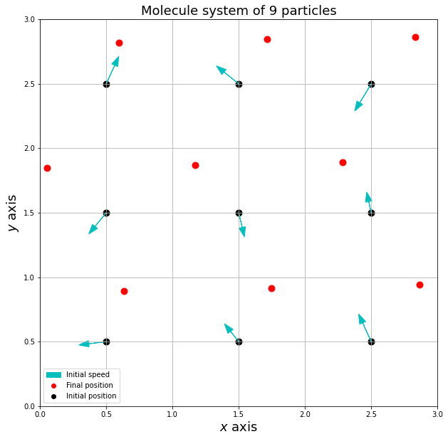
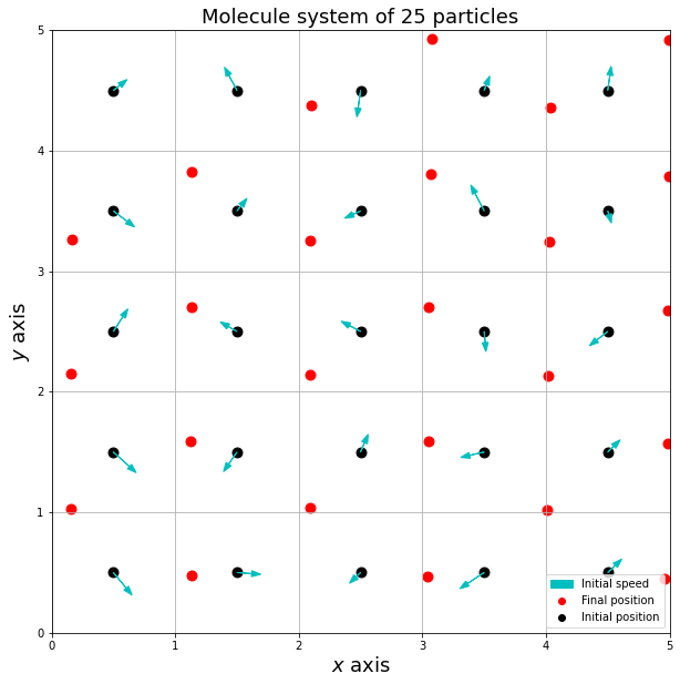
The simulation results are very interesting, the particles spontaneously go into a ground state and form a lattice pattern:


For more details on this project, you can read my report.